Kriging as gaussian processes

This example shows how our kriging package can be used for gaussian processes as in scikit-learn.

# sphinx_gallery_thumbnail_number = 2

Import packages

from pylawr.grid.unstructured import UnstructuredGrid
from pylawr.remap import kernel as k_ops
from pylawr.remap import SimpleKriging, OrdinaryKriging

import numpy as np
import matplotlib.pyplot as plt
import xarray as xr

We have to write a function to use UnstructuredGrid for Gaussian processes.

def append_lat(lon):
    lat = np.zeros_like(lon)
    return np.stack([lat, lon], axis=1)

rnd = np.random.RandomState(0)

Define data

x_train = rnd.uniform(high=15, size=100)
y_train = np.sin(x_train)
y_train += 3 * (0.5 - rnd.rand(*x_train.shape))
grid_train = UnstructuredGrid(append_lat(x_train), center=(0, 0, 0))
grid_train._earth_radius = 360/2/np.pi

x_linspace = np.linspace(0, 20, 1000)
y_linspace = np.sin(x_linspace)

grid_linspace = UnstructuredGrid(append_lat(x_linspace), center=(0, 0, 0))
grid_linspace._earth_radius = 360/2/np.pi

train_data = xr.DataArray(
    y_train.reshape(1, -1),
    coords=dict(
        time=[0, ],
        grid=x_train
    ),
    dims=['time', 'grid']
)
train_data = train_data.lawr.set_grid_coordinates(grid_train)

Define kernels

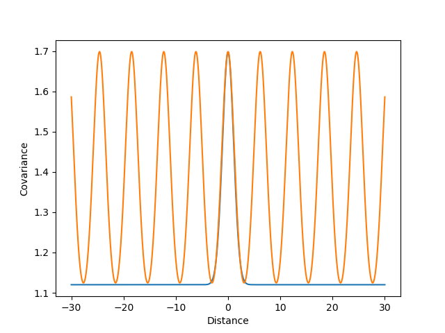
Define and plot kernels

rbf_data_kernel = k_ops.gaussian_rbf(length_scale=1.08, stddev=0.76)
rbf_noise_kernel = k_ops.WhiteNoise(rbf_data_kernel.placeholders[0],
                                    noise_level=1.12)
rbf_kernel = rbf_data_kernel+rbf_noise_kernel

scikit_data_kernel = k_ops.exp_sin_squared(length_scale=1.53, periodicity=6.15)
scikit_noise_kernel = k_ops.WhiteNoise(scikit_data_kernel.placeholders[0],
                                       noise_level=0.699)
scikit_kernel = scikit_data_kernel+scikit_noise_kernel

distances = np.linspace(-30, 30, 1000)

fig, ax = plt.subplots()
ax.plot(distances, rbf_kernel.diag(distances), label='RBF Kernel')
ax.plot(distances, scikit_kernel.diag(distances), label='Scikit Kernel')
ax.set_xlabel('Distance')
ax.set_ylabel('Covariance')
plt.show()

Fit kriging instances

gp_rbf = SimpleKriging(kernel=rbf_kernel, n_neighbors=20, alpha=1E-10)
gp_scikit = SimpleKriging(kernel=scikit_kernel, n_neighbors=100, alpha=1E-10)
gp_ord = OrdinaryKriging(kernel=scikit_kernel, n_neighbors=20, alpha=1E-10)

gp_rbf.fit(grid_train, grid_linspace)
gp_scikit.fit(grid_train, grid_linspace)
gp_ord.fit(grid_train, grid_linspace)

Plot predictions of kriging

pred_rbf = (gp_rbf.remap(train_data), np.sqrt(gp_rbf.covariance))
pred_scikit = (gp_scikit.remap(train_data), np.sqrt(gp_scikit.covariance))
pred_ord = (gp_ord.remap(train_data), np.sqrt(gp_ord.covariance))

/home/docs/checkouts/readthedocs.org/user_builds/pylawr/conda/stable/lib/python3.11/site-packages/xarray/core/coordinates.py:41: FutureWarning: Updating MultiIndexed coordinate 'grid_cell' would corrupt indices for other variables: ['grid_lat', 'grid_lon']. This will raise an error in the future. Use `.drop_vars({'grid_lat', 'grid_lon', 'grid_cell'})` before assigning new coordinate values.
  self.update({key: value})

fig, ax = plt.subplots(figsize=(10, 5))
ax.scatter(x_train, y_train, c='k', label='data')
ax.plot(x_linspace, y_linspace, color='0.1', lw=2, label='True')
ax.plot(x_linspace, pred_scikit[0].values.ravel(), color='turquoise',
        lw=2, label='GP Scikit')
plt.fill_between(x_linspace, pred_scikit[0].values.ravel() - pred_scikit[1],
                 pred_scikit[0].values.ravel() + pred_scikit[1],
                 color='turquoise',
                 alpha=0.2)
ax.plot(x_linspace, pred_ord[0].values.ravel(), color='royalblue', lw=2,
        label='GP Scikit (Ordinary Kriging)')
plt.fill_between(x_linspace, pred_ord[0].values.ravel() - pred_ord[1],
                 pred_ord[0].values.ravel() + pred_ord[1], color='royalblue',
                 alpha=0.2)
ax.plot(x_linspace, pred_rbf[0].values.ravel(), color='darkorange', lw=2,
        label='GP RBF')
plt.fill_between(x_linspace, pred_rbf[0].values.ravel() - pred_rbf[1],
                 pred_rbf[0].values.ravel() + pred_rbf[1], color='darkorange',
                 alpha=0.2)
ax.set_xlabel('data')
ax.set_ylabel('target')
ax.set_xlim(0, 20)
ax.set_ylim(-4, 4)
plt.legend(loc="best",  scatterpoints=1, prop={'size': 8})
plt.show()

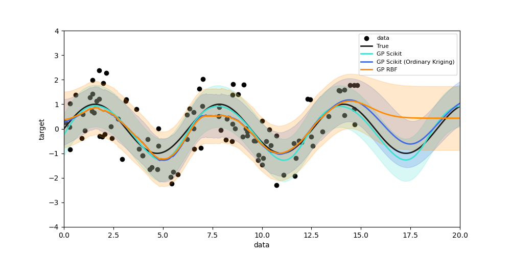
We can see that the scikit-learn kernel solution with all data points is the smoothest solution of all three. If localize the kriging, then we get a damped and more local prediction. The difference between RBF kernel and sine kernel is shown after 15, where the prior of the RBF kernel is 0, while the sine kernel is a sine function.